Discretization
-
To discretize input sequence need a step size representing .
-
One choice for discretization is a bilinear transform.
def discretize(A, B, C, step):
    I = np.eye(A.shape[0])
    BL = inv(I - (step / 2.0) * A)
    Ab = BL @ (I + (step / 2.0) * A)
    Bb = (BL * step) @ B
    return Ab, Bb, C
Discretized SSM as RNN
- Once discretized with step , the SSM can be viewed as a linear RNN,
def scan_SSM(Ab, Bb, Cb, u, x0):
    def step(x_k_1, u_k):
        x_k = Ab @ x_k_1 + Bb @ u_k
        y_k = Cb @ x_k
        return x_k, y_k

    return jax.lax.scan(step, x0, u)
Tangent: A Mechanics Example
-
Example from mechanics, mass on a spring
- forward position
- force is applied to this mass
- parameterized by mass (), spring constant (), friction constant ()
Tangent: A Mechanics Example [Matrix form]
def example_mass(k, b, m):
    A = np.array([[0, 1], [-k / m, -b / m]])
    B = np.array([[0], [1.0 / m]])
    C = np.array([[1.0, 0]])
    return A, B, C
Tangent: A Mechanics Example (with force)
@partial(np.vectorize, signature="()->()")
def example_force(t):
    x = np.sin(10 * t)
    return x * (x > 0.5)
def example_ssm(L=100):
    ssm = example_mass(k=40, b=5, m=1)

    # L samples of u(t).
    step = 1.0 / L
    ks = np.arange(L)
    u = example_force(ks * step)
    y = scan_SSM(*ssm, u)

Training SSMs
- Our Goal: Train a neural network with SSMs
- SSM RNNs: Fast for generation, but slow for training
Key Properties
- SSM CNNs: Slow for generation, but fast for training
- Initilization
SSMs as wide CNNs
- "Unroll" the RNN representation
SSMs as wide CNNs
- Form a -length kernel
def K_conv(Ab, Bb, Cb, L):
    return np.array(
        [(Cb @ matrix_power(Ab, l) @ Bb).reshape() for l in range(L)]
    )
SSMs as wide CNNs
- Apply as a (non-cicular) convolution
def non_circular_convolution(u, K, nofft=False):
    if nofft:
        return convolve(u, K, mode="full")[: u.shape[0]]
    else:
        ud = np.fft.rfft(np.pad(u, (0, K.shape[0])))
        Kd = np.fft.rfft(np.pad(K, (0, u.shape[0])))
        return np.fft.irfft(ud * Kd)[: u.shape[0]]
- training through FFT
Initialization with HiPPO
- Fast training, but random init does terribly. MNIST classification benchmark .
- HiPPO initialization of improves this number to
def make_HiPPO(N):
    def v(n, k):
        if n > k:
            return np.sqrt(2 * n + 1) * np.sqrt(2 * k + 1)
        elif n == k:
            return n + 1
        else:
            return 0
    mat = [[v(n, k) for k in range(1, N + 1)] for n in range(1, N + 1)]
    return -np.array(mat)
HiPPO Intuition Sketch
- Recall is an -dimensional hidden representation of an -step signal
- HiPPO approximates state as Legendre coefficients representing .
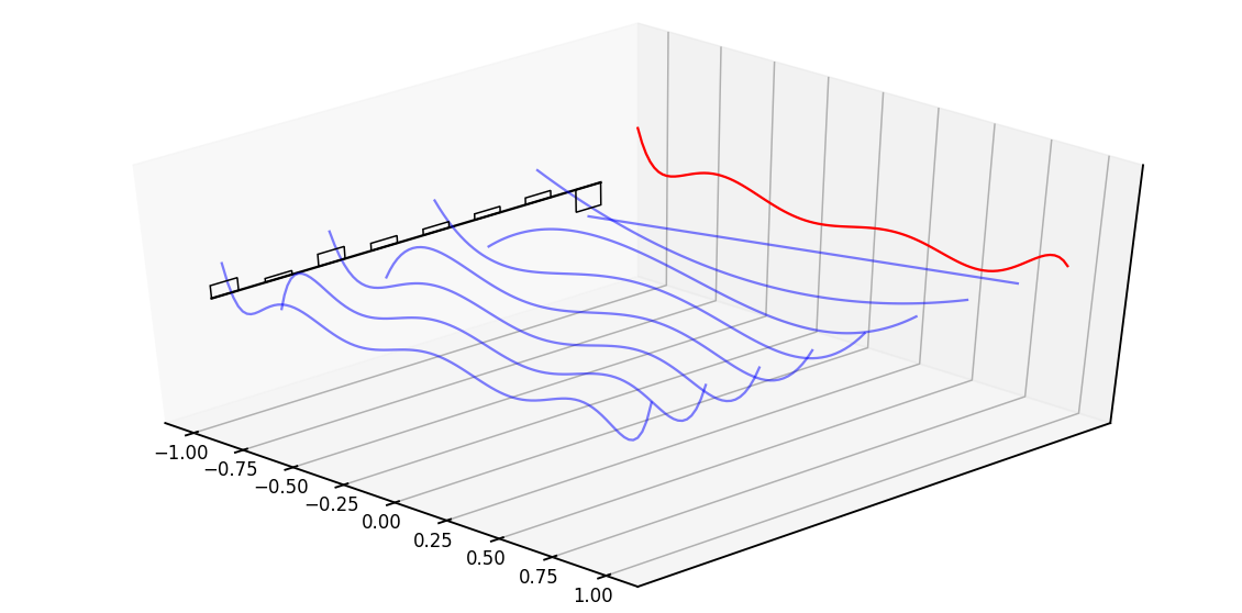
def example_legendre(N=8):
    u = (np.random.rand(N) - 0.5) * 2
    t = np.linspace(-1, 1, 100)
    x = numpy.polynomial.legendre.Legendre(u)(t)
Tangent: Neat JAX things.
- Everything is a modular testable function
- So far - no parameter, batches, NN nonsense
- In fact, mostly scalar modeling.
SSM Network Layer
- SSM layer with Flax (still scalar!)
class SSMLayer(nn.Module):
    A: np.DeviceArray  # HiPPO
    N, L: int

    def setup(self):
        self.B = self.param("B", lecun_normal(), (self.N, 1))
        self.C = self.param("C", lecun_normal(), (1, self.N))
        self.step = np.exp(self.param("log_step", log_step_initializer(), (1,)))

        # Conv created each time during training
        self.ssm = discretize(self.A, self.B, self.C, step=self.step)
        self.K = K_conv(*self.ssm, self.L)

    def __call__(self, u):
        return non_circular_convolution(u, self.K)
Lifting SSM Layer
- Lift to copies
nn.vmap(
    layer, in_axes=1, out_axes=1,
    variable_axes={"params": 1}, # New Params
    split_rngs={"params": True},
)
- Over batches
nn.vmap(
    layer, in_axes=0, out_axes=0,
    variable_axes={"params": None}, # Shared Params
    split_rngs={"params": False},
)
- Put into a stack of layers (similar to Transformers)
SSM RNN Layer
- Alternative SSM layer with Flax Caching
class SSMRNNLayer(nn.Module):
    A: np.DeviceArray  # HiPPO
    N, L: int

    def setup(self):
        self.B = self.param("B", lecun_normal(), (self.N, 1))
        self.C = self.param("C", lecun_normal(), (1, self.N))
        self.step = np.exp(self.param("log_step", log_step_initializer(), (1,)))
        self.ssm = discretize(self.A, self.B, self.C, step=self.step)
        self.x_k_1 = self.variable("cache", "cache_x_k", np.zeros, (self.N,))

    def __call__(self, u):
        x_k, y_s = scan_SSM(*self.ssm, u[:, np.newaxis], self.x_k_1.value)
        if self.is_mutable_collection("cache"):
           self.x_k_1.value = x_k
        return y_s.reshape(-1).real + self.D * u
Part 2: S4
Issue: Calculating
- Unfortunately, this step is a problem.
def K_conv(Ab, Bb, Cb, L):
    return np.array(
        [(Cb @ matrix_power(Ab, l) @ Bb).reshape() for l in range(L)]
    )
-
Main contribution of S4 is to fix this function.
-
Today: quick sketch of how it works
Two S4 Tricks
See blog post for full details. Here are two neat JAX tricks.
-
Instead of computing directly, S4 evaluates its truncated generating function.
- This becomes a functional
vmapin JAX.
- This becomes a functional
-
In order to evalute the generating function it computes a Cauchy kernel .
- This is intractable in Torch, but is jitted out in JAX.
Trick 1. SSM Generating Functions
The truncated SSM generating function at node with truncation is
def K_gen_naive(Ab, Bb, Cb, L):
    K = K_conv(Ab, Bb, Cb, L)
    return lambda z: np.sum(K * (z ** np.arange(L)))
Trick 1. SSM Generating Functions
We can recover the kernel through a z-transform at the roots of unity
and inverse fourier transformation.
def conv_from_gen(gen, L):
    Omega_L = np.exp((-2j * np.pi) * (np.arange(L) / L))
    atRoots = jax.vmap(gen)(Omega_L)
    return np.fft.ifft(atRoots, L).reshape(L).real
Trick 1. SSM Generating Functions
Simplifying the generating function allows us to avoid calling K_conv
def K_gen_inverse(Ab, Bb, Cb, L):
    I = np.eye(Ab.shape[0])
    Ab_L = matrix_power(Ab, L)
    Ct = Cb @ (I - Ab_L)
    return lambda z: (Ct.conj() @ inv(I - Ab * z) @ Bb).reshape()
Trick 2. Exploiting Structure
Under a diagonal assumption on you can further reduce the generating function to the following kernel form,
where is a constant, and is a function of .
-
However the transform of this function is memory and compute-intensive.
- different , different
- Instantiating full tensor is intractable
- Libraries like KeOps avoid this issue
Trick 2. Exploiting Structure
In JAX we can rely on the JIT to take care of this for us.
- JIT handles the fusion of the sum term
@partial(np.vectorize, signature="(c),(),(c)->()")
def cauchy_dot(v, omega, lambd):
    return (v / (omega - lambd)).sum()
- JAX
remathandles cases of very long sequences.
jax.remat(cauchy_dot)
Part 3: S4 in Practice
Training S4
- So far: tested code for training S4 as a CNN and running it as an RNN.
- MNIST classification and CIFAR classification (by pixel) are strong.

Goal
- Generate extremely long sequences.

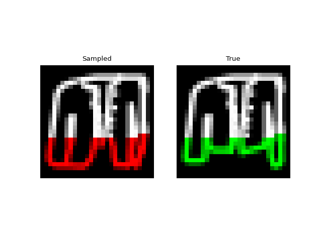
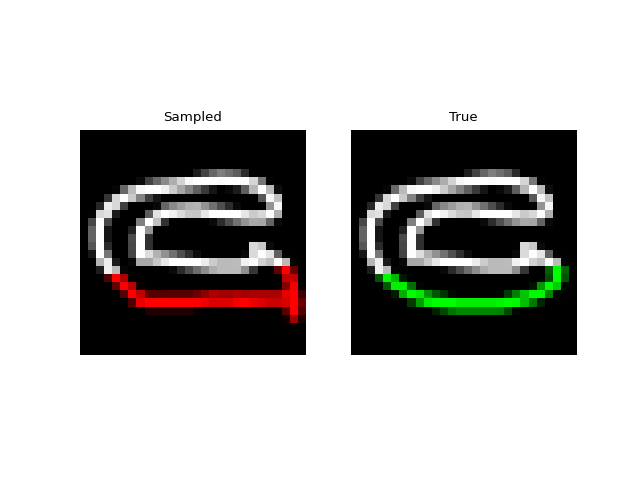
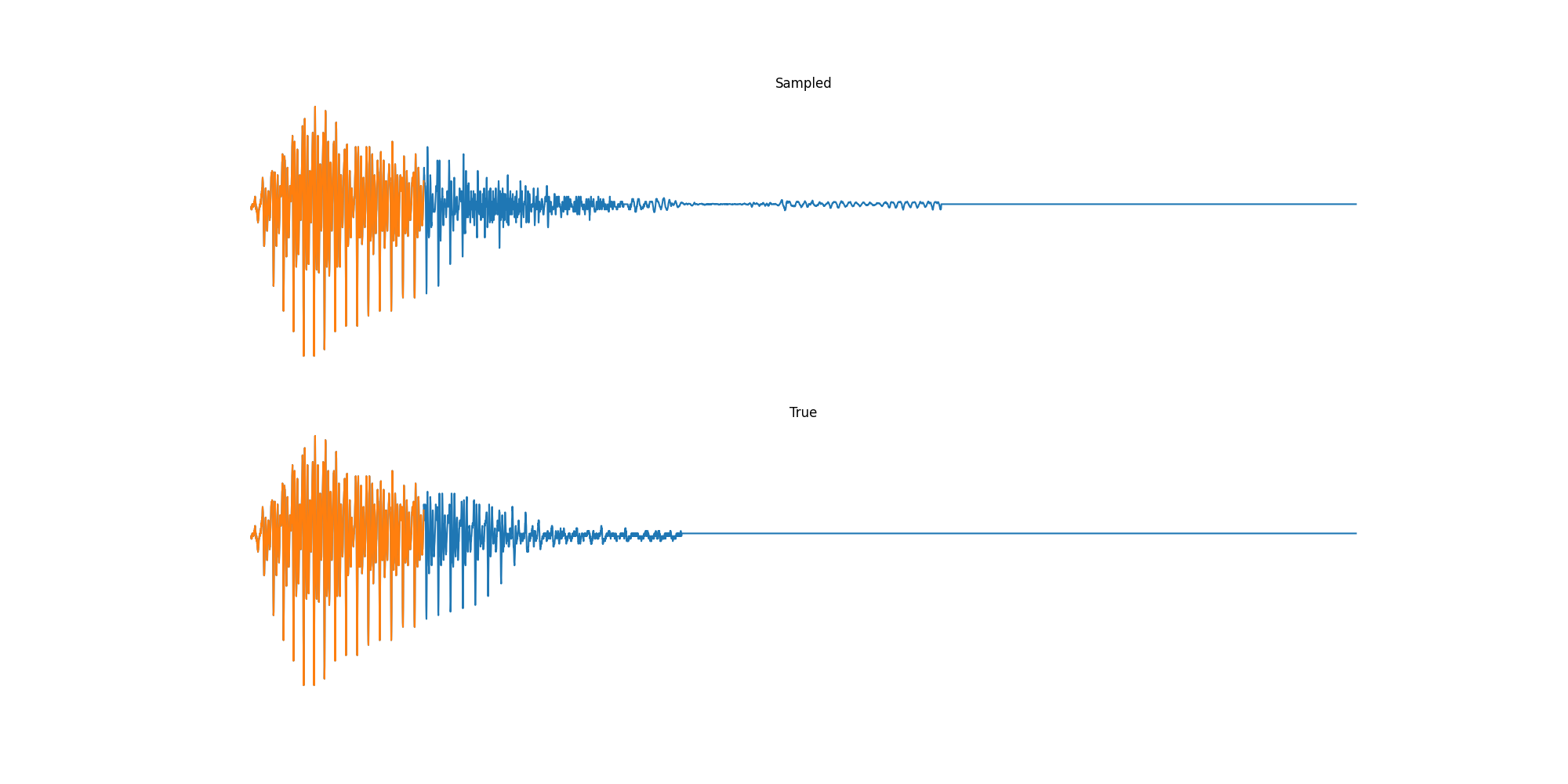
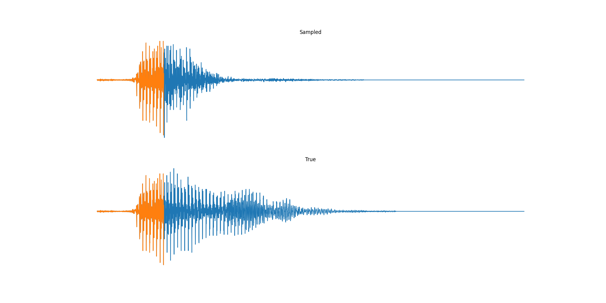
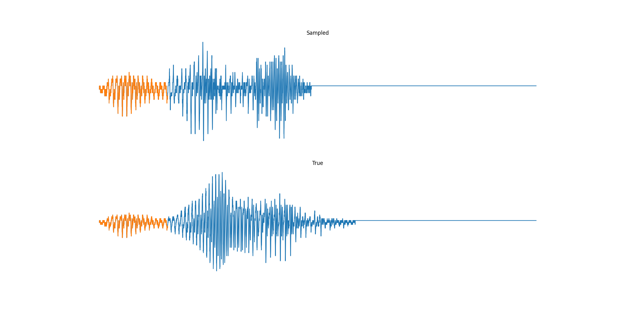
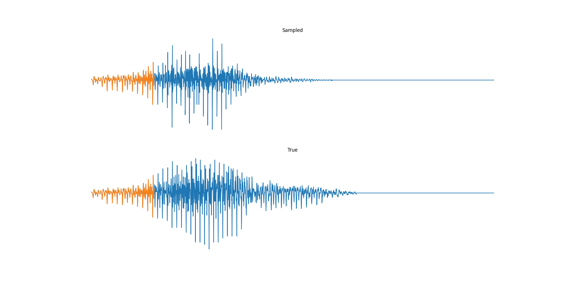
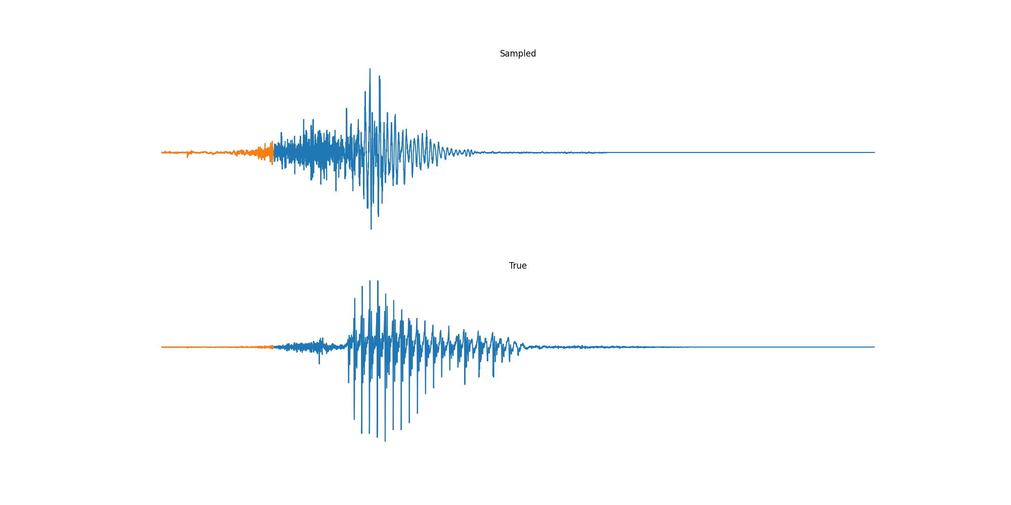
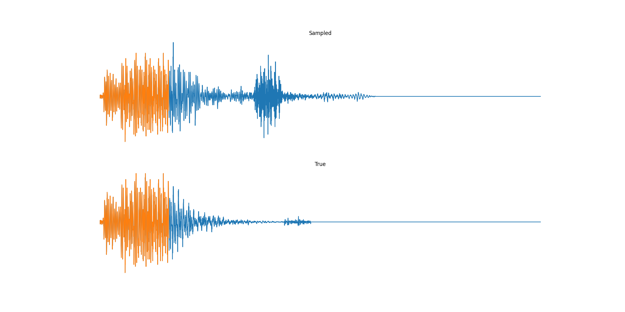
- Expreriments on MNIST, QuickDraw, SpeechCommands
S4 Model
Training to Generate by Pixeal
Code to sample from the RNN
def sample(model, params, prime, cache, x, start, end, rng):
    def loop(i, cur):
        x, rng, cache = cur
        r, rng = jax.random.split(rng)
        out, vars = model.apply(
            {"params": params, "cache": cache},
            x[:, np.arange(1, 2) * i],
            mutable=["cache"],
        )

        def update(x, out):
            p = jax.random.categorical(r, out[0])
            return x.at[i + 1, 0].set(p)

        x = jax.vmap(update)(x, out)
        return x, rng, vars["cache"].unfreeze()

    return jax.lax.fori_loop(start, end, loop, (x, rng, cache))[0]
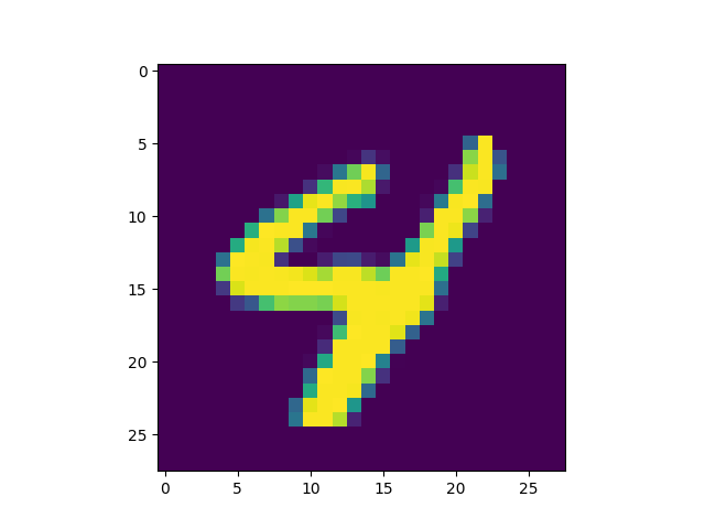
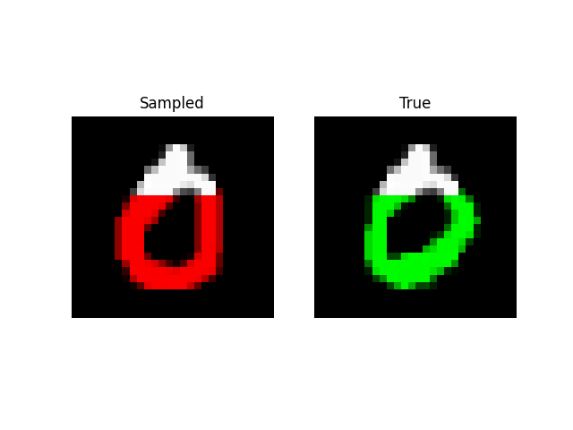
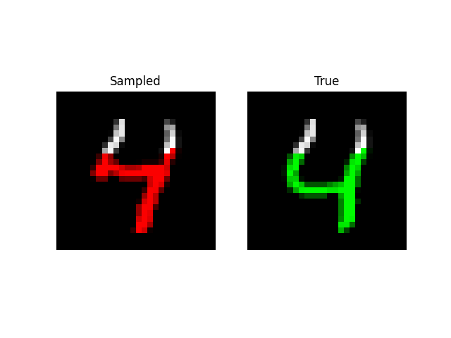
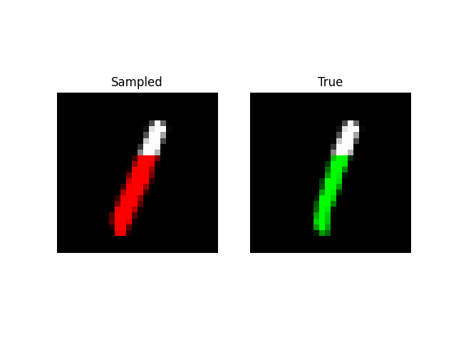
Generating by Pixel
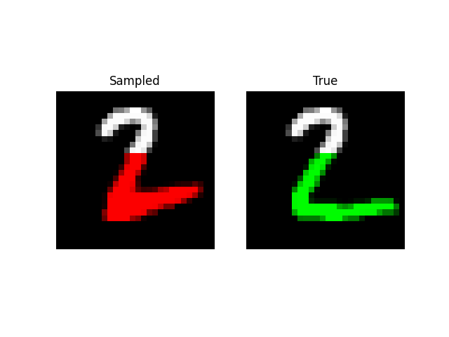
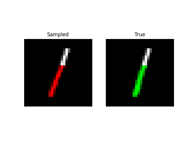
Prefix Generation
Experiments: QuickDraw


Experiments: Sound
Conclusion & Future Work
Conclusion (on JAX)
-
JAX really signs at modular mathematical code.
-
JAX JIT makes some hard code trivial.
-
Lifting in Flax
New Paper - Diagonal State Spaces.
# Replaces Part 2.
def complex_softmax(x, eps=1e-7):
    def reciprocal(x):
        return x.conj() / (x * x.conj() + eps)

    x2 = x - x[np.argmax(x.real)]
    e = np.exp(x2)
    return e * reciprocal(np.sum(e))

def dss_kernel(W, Lambda, L, step):
    P = (step * Lambda)[:, None] * np.arange(L)
    S = jax.vmap(complex_softmax)(P)
    return ((W / Lambda) @ S).ravel().real

def dss_ssm(W, Lambda, L, step):
    N = Lambda.shape[0]
    Abar = np.diag(np.exp(Lambda * step))
    b = jax.vmap(lambda l:
                 1 / (l * (np.exp(l * np.arange(L) * step)).sum()))
    Bbar = b(Lambda).reshape(N, 1)
    Cbar = W.reshape(1, N)
    return (Abar, Bbar, Cbar)
Thank You
-
Huge thanks to Albert Gu and Karan Goel, who were super helpful in putting this together. Their paper and codebase.
-
Ankit Gupta for helping with his DSS model
-
Thanks to Conner Vercellino, Laurel Orr, Ankit Gupta, Ekin Akyürek, Saurav Maheshkar